This notebook is a part of an assignment to the course Advanced Data Science Capstone, which is a part of Advanced Data Science with IBM Specialization. According to the course description, "capstone project completer has proven a deep understanding on massive parallel data processing, data exploration and visualization, advanced machine learning and deep learning and how to apply his knowledge in a real-world practical use case where he justifies architectural decisions, proves understanding the characteristics of different algorithms, frameworks and technologies and how they impact model performance and scalability."
Introduction
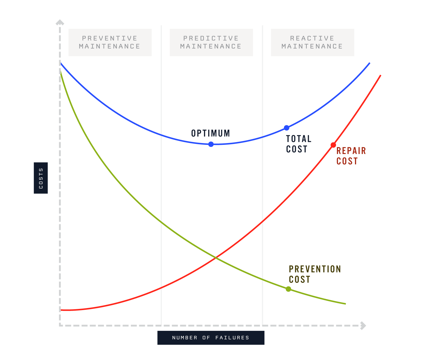
Aim of the project is to minimize the maintenance costs by predicting machine failures based on the measurement data. Subject is important not only in academic world but also in real life. Preventive maintenance costs money because healthy parts of a machine are changed without sufficient knowledge could they be used longer time, and reactive maintenance costs money due to the uncontrolled interruption in production. It would be optimal to use the measurement data to assess the condition of the device and to take the necessary maintenance at the right time.
Source: https://www.losant.com/hs-fs/hubfs/Blog/machine_learning/googleML-blogImage-02.png
Data set
This project uses FEMTO Bearing Data Set, which is available on Internet for free of charge. Data set contains measurement data for 17 different bearing: Bearing1_1, Bearing1_2, Bearing1_3, Bearing1_4, Bearing1_5, Bearing1_6, Bearing1_7, Bearing2_1, Bearing2_2, Bearing2_3, Bearing2_4, Bearing2_5, Bearing2_6, Bearing2_7, Bearing3_1, Bearing3_2, Bearing3_3.
In this project, only one bearing measurement is used, Bearing2_1. Each measurement contains approximate 1000 csv files of accelerometer data and 150 csv files of temperature measurement data. Only accelerometer data is used to determine the condition of the bearing. Each acceleration measurement contains 2560 data points and the sampling rate is 25 kHz, thus every measurement is about 0.1 seconds. Measurement is repeated every 10 seconds until bearing fails.
Other studies made from the data set:
Data Quality Assessment
Data quality assessment (DQA) is the process of scientifically and statistically evaluating data in order to determine whether they meet the quality required for projects or business processes and are of the right type and quantity to be able to actually support their intended use.

Image source: http://www.dataintegration.ninja/taking-a-dive-into-data-quality-assessment-approaches.
In this project, data quality was verified by visual inspection. The method is sufficient considering the nature of the project.
Data exploration
To get an idea of the data, let us open the first sample file to study the signal in the beginning of the test. At this stage, the obvious assumption is that bearing is healty.
import pandas as pd
import matplotlib.pylab as plt
import seaborn as sns
import numpy as np
%matplotlib inline
filename = "FEMTOBearingDataSet/Bearing2_1/acc_00001.csv"
data = pd.read_csv(filename, names=["h", "m", "s", "us", "ax", "ay"])
data.head()
First 4 columns are for time stamp and columns 4 and 5 are accelerometer results, in vertical and horizontal directions. The first 300 samples looks following:
fig, (ax1, ax2) = plt.subplots(2, 1, figsize=(12.8, 7.2))
data.head(300)["ax"].plot(ax=ax1, color="k")
data.head(300)["ay"].plot(ax=ax2, color="k")
for ax in (ax1, ax2):
    ax.set_xlim(0, 300)
    ax.grid()
ax1.set_title("Acceleration in vertical direction")
ax2.set_title("Acceleration in horizontal direction");

Correlation between two channels:
corr = data[["ax", "ay"]].corr()
corr
There is weak negative correlation between acceleration:
import seaborn as sns
fig, ax = plt.subplots(figsize=(7.2, 7.2))
g = sns.regplot("ax", "ay", data=data, color="k", marker=".")
ax.set_xlabel("horizontal acceleration")
ax.set_ylabel("vertical acceleration");
ax.set_title("correlation between columns, r = %0.2f" % corr["ax"]["ay"]);

Data visualization
Let us also compare visually how does the measurement data look before and after failure.
def read_data(no):
    """ Given file number, read data to Pandas DataFrame. """
    names = ["h", "m", "s", "us", "ax", "ay"]
    filename = "FEMTOBearingDataSet/Bearing2_1/acc_%05i.csv" % no
    return pd.read_csv(filename, names=names)

data1 = read_data(1)
data911 = read_data(911)

fig, (ax1, ax2) = plt.subplots(2, 1, figsize=(12.8, 7.2))
data1.head(300)["ay"].plot(ax=ax1, color="k")
data911.head(300)["ay"].plot(ax=ax2, color="k")
for ax in (ax1, ax2):
    ax.grid()
    ax.set_xlim(0, 300)
ax1.set_title("Healty bearing")
ax2.set_title("Failed bearing")
plt.tight_layout()

What can be immediately said about the data that in the beginning of test vibration is between -1 ... 1 and at the end it's more like -5 ... 5. There is also high spikes in data.
To get better idea of the structure of the data, we can plot the distributions:
fig, ax = plt.subplots(figsize=(7.2, 7.2))
sns.distplot(data1["ay"], ax=ax, label="Sample 1")
sns.distplot(data911["ay"], ax=ax, label="Sample 911")
ax.set_title("Vertical acceleration of bearing in the beginning and end of test")
ax.set_xlim(-10, 10)
ax.grid()
ax.legend();

data1["ay"].std(), data911["ay"].std()
Clearly, a standard deviation of the vibration is increasing from 0.26 to 2.21 during the test, which could be used to determine the failure of the bearing.
Feature engineering
It should be noted, that so far we have been stuing only the vertical acceleration of the data. But there is another measurement also, namely acceleration in horizontal direction. Together, channels form a vector. This vector we can conveniently present in a polar coordinate system, because in general, we are more interested about the amplitude of the signal rather than direction.

data1["r"] = np.sqrt(data1["ax"]**2 + data1["ay"]**2)
data1.head()
data911["r"] = np.sqrt(data911["ax"]**2 + data911["ay"]**2)
data911.head()
fig, ax = plt.subplots(figsize=(7.2, 7.2))
sns.distplot(data1["r"], ax=ax, label="Sample 1")
sns.distplot(data911["r"], ax=ax, label="Sample 911")
ax.set_title("Acceleration amplitude of bearing in the beginning and end of test")
ax.set_xlim(0, 10)
ax.grid()
ax.legend()

It should be noted, that standard deviation is no more relevant measure because after feature engineering, samples are not normally distributed! It turns out, that magnitude a of vector forms a Rayleigh distribution.
X1 = np.random.randn(100000)
X2 = np.random.randn(100000)
Xr = np.sqrt(X1**2 + X2**2)
fig, (ax1, ax2) = plt.subplots(1, 2, figsize=(12.8, 7.2))
sns.distplot(X1, ax=ax1)
sns.distplot(Xr, ax=ax2)
ax1.grid()
ax2.grid()
ax1.set_title("Normal distribution X ~ N(1,0)")
ax2.set_title("Rayleigh distribution X ~ R(0,1)")

Parameter estimation can be done e.g. scipy.stats:
from scipy.stats import rayleigh
rayleigh.fit(Xr)
d1 = rayleigh.fit(data1["r"])
d1
d911 = rayleigh.fit(data911["r"])
d911
rvs1 = rayleigh(loc=d1[0], scale=d1[1])
rvs911 = rayleigh(loc=d911[0], scale=d911[1])
fig, ax = plt.subplots(figsize=(7.2, 7.2))
sns.distplot(data1["r"], ax=ax, kde=True, label="Sample 1")
sns.distplot(data911["r"], ax=ax, kde=True, label="Sample 911")
ax.set_title("Acceleration amplitude of bearing in the beginning and end of test")
ax.set_xlim(0, 10)
ax.grid()
x = np.linspace(0, 10)
ax.plot(x, rvs1.pdf(x), label="R(%0.2f, %0.2f)" % d1)
ax.plot(x, rvs911.pdf(x), label="R(%0.2f, %0.2f)" % d911)
ax.legend()

It actually looks a bit that when the bearing fails, the data is not Rayleigh-distributed.
Another, maybe more "engineering" approach, is to, instead of calculating statistical properties of distribution, to calculate some energy-based quantity like root mean square of acceleration. If we calculate the spectral density of the signal, we could then esimate energy in different frequency areas to detect failure. To keep things simple, we do calculate the overall energy of the random vibration and not study it's energy spectrum.
N = len(data1)
rms1 = np.sqrt(1/N*np.sum(data1["r"]**2))
rms911 = np.sqrt(1/N*np.sum(data911["r"]**2))
rms1, rms911
Yet another feature could be the absolute maximum of the signal. While it clearly indicates high amplitude peaks in data, it's somewhat sensitive to measurement errors and thus not very reliable alone.
absmax1 = np.max(np.abs(data1["r"]))
absmax911 = np.max(np.abs(data911["r"]))
absmax1, absmax911
"Traditional" machine learning approach: k-means clustering
Before going into deep learning, let's try something more traditional, yet still machine learning approach, including the feature engineering described above. For each sample file, let's calculate rms of acceleration and absolute maximum of acceleration, and use some simple unsupervised learning technique, like k-means clustering, to determine the clusters of healty and broken bearings.
def extract_features(no):
    """ Extract features from sample file `no`. """
    data = read_data(no)
    r = np.sqrt(data["ax"]**2 + data["ay"]**2)
    N = len(r)
    rms = np.sqrt(1/N*np.sum(r**2))
    absmax = np.max(np.abs(r))
    return [rms, absmax]

extract_features(1), extract_features(911)
X = np.array([extract_features(i+1) for i in range(911)])
fig, (ax1, ax2) = plt.subplots(2, 1, figsize=(12.8, 7.2))
ax1.plot(np.arange(911)+1, X[:,0])
ax1.set_ylabel("Root mean square of acceleration")
ax1.grid()
ax2.plot(np.arange(911)+1, X[:,1])
ax2.set_xlabel("Sample file number")
ax2.set_ylabel("Absolute maximum of acceleration")
ax2.grid()
ax1.set_xlim(1, 911)
ax2.set_xlim(1, 911)

So what we can say about this experiment, is that rms levels are continuously changing during the test and there is no clear "limit", where failure of bearing begins. Sudden spikes in the absolution maximum of the acceleration could either indicate failure or measurement error.
fig, ax = plt.subplots(figsize=(7.2, 7.2))
ax.scatter(X[:,0], X[:,1], facecolor="k", color="k", s=50)
ax.set_xlabel("rms of acceleration")
ax.set_ylabel("absmax of acceleration")
ax.grid();

Here is our unlabelled data, and next we should find decision boundary to determine faulty data, using k-means clustering.
from sklearn.pipeline import Pipeline
from sklearn.preprocessing import StandardScaler
from sklearn.cluster import KMeans

scaler = StandardScaler()
kmeans = KMeans(n_clusters=2)
pipe = Pipeline(steps=[('scale', scaler),
                       ('kmeans', kmeans)])

pipe.fit(X)
Now, let's use k-means clustering to find a "decision boundary" for data:
healthy, = np.where(kmeans.labels_ == 0)
damaged, = np.where(kmeans.labels_ == 1)
fig, ax = plt.subplots(figsize=(7.2, 7.2))
ax.scatter(X[healthy,0], X[healthy,1], s=50, color="k", facecolor="g")
ax.scatter(X[damaged,0], X[damaged,1], s=50, color="k", facecolor="r")
ax.set_xlabel("rms of acceleration")
ax.set_ylabel("absmax of acceleration")
ax.grid();

The first file, where indicator gives 1 (failure), is
np.where(kmeans.labels_ == 1)[0][0] + 1
data507 = read_data(507)
data507["r"] = np.sqrt(data507["ax"]**2 + data507["ay"]**2)
time = np.arange(2560)/25.0
fig, ax = plt.subplots(1, 1, figsize=(12.8, 7.2))
ax.plot(time, data507["r"])
ax.grid()
ax.set_title("Acceleration amplitude, file 507")
ax.set_ylabel("Acceleration amplitude")
ax.set_xlabel("Time [ms]")
ax.set_xlim(time.min(), time.max());

np.save("kmeans.npy", kmeans.labels_)
To sum up, and to make this study more comparable with other algorithms, let's find out how long test lasted until the first symptoms of failure:
print(data1.head(1)[["h", "m", "s"]])
print(data507.head(1)[["h", "m", "s"]])
print(data911.head(1)[["h", "m", "s"]])
t0 = pd.Timestamp("8:14:15")
tf = pd.Timestamp("9:38:35")
t1 = pd.Timestamp("10:45:55")
print("Test total duration: %i seconds" % (t1-t0).seconds)
print("First failure at:    %i seconds" % (t1-tf).seconds)
Deep learning approach: LSTM Autoencoder
Before it was seen, that when using "traditional" machine learning approach, a lot of decisions needed to made in order to find a good indicator for estimating bearing failure. First we needed to do feature engineering, where we made a coordinate transform to polar coordinates to get the amplitude of acceleration and after that, we extracted two features, namely root mean square and absolutely maximum value of acceleration, which was then used to predict a bearing failure. This all needed quite a lot of domain expertise and finally, made decisions have significant impact on the end result. What if there exists a way to simplify the pipeline, just throw data in and get the results? Next, a deep learning approach is used, which (hopefully) replaces all these cumbersome and laborius tasks and simplifies analysis.
The idea is to train LSTM Autoencoder to the measured accelerometer data and detect bearing failure based on the relative change of the loss function during training. It is assumed that LSTM can model the dynamics of the system without any problems in normal operating conditions, until the damage in the bearing is adding some additional terms into vibration data and causing inaccuracy to autoencoder. The inaccuracy of the encoder is then measured using "loss", \begin{equation} \mathcal{L}\left(\boldsymbol{x},\boldsymbol{y}\right)=\left\Vert \boldsymbol{x}-\boldsymbol{y}\right\Vert ^{2}, \end{equation} which is compared to the base level. It is expected that when autoencoder is not capable to reproduce input data accurately, a loss is increasing and thus indicating that the dynamical behavior of bearing has been changed due to damage.
Further reading about the technologies used in this project:
import pandas as pd
import numpy as np
from keras.models import Sequential
from keras.layers import Dense, LSTM
from keras.callbacks import Callback
import matplotlib.pylab as plt
import time
%matplotlib inline
Setup is the following: we use LSTM neural network with 5 nodes and train with batch size of 64.
class LossHistory(Callback):

    def on_train_begin(self, logs={}):
        self.losses = []

    def on_batch_end(self, batch, logs={}):
        self.losses.append(logs.get("loss"))

timesteps = 16
dim = 2
loss_history = LossHistory()
model = Sequential()
model.add(LSTM(20, input_shape=(timesteps, dim),
               return_sequences=True))
model.add(Dense(2))
model.compile(loss="mae", optimizer="adam")
We are ready to go. Here we loop each file and each file is containing approx. 0.1 seconds of accelerometer data. Train the model to understand the data, and measure loss for each training session.
def train(no, epochs=1):
    """ Train data and return mean loss for file number `no`. """
    names = ["h", "m", "s", "us", "ax", "ay"]
    filename = "FEMTOBearingDataSet/Bearing2_1/acc_%05i.csv" % no
    data = pd.read_csv(filename, names=names)
    N = len(data)
    X = np.array(data[["ax", "ay"]])
    X = X.reshape(N//timesteps, timesteps, dim)
    model.fit(X, X, batch_size=32,
              epochs=epochs,
              validation_data=(X, X),
              verbose=0, shuffle=False,
              callbacks=[loss_history])
    loss = loss_history.losses
    return np.mean(loss)
t0 = time.time()
mean_loss = []
for i in range(1, 912):
    mean_loss.append(train(i))
mean_loss = np.array(mean_loss)
dt = time.time() - t0
print("Training completed in %0.1f seconds" % dt)
fig, ax = plt.subplots(figsize=(12.8, 3.6))
ax.plot(mean_loss, "-k")
ax.set_title("Mean loss")
ax.grid()
ax.set_xlim(0, 911);

To make detection more robust, loss should be compared to some base level, for example by taking moving average from loss and calculating how much does the loss function differ related to this base level. We also should skip the first results from the estimator, because
d = pd.DataFrame({"loss": mean_loss}, index=np.arange(1, 912))
d["baselevel"] = d.rolling(10).mean()
d["pct_change"] = (d["loss"]-d["baselevel"])/d["baselevel"]
fig, ax = plt.subplots(figsize=(12.8, 3.6))
d["pct_change"].plot(ax=ax, color="k", label="pct_change to base level")
d["baselevel"].plot(ax=ax, color="r", label="base level")
ax.grid()
ax.legend()
ax.set_title("Bearing malfunction indicator; change of loss function with respect to the base level");

Say, that over 100 % change in loss function compared to the base level is clear indication of change in dynamical behavior of bearing:
d[d["pct_change"] > 1.0].head()
Based on this, I would say that bearing is starting to malfunction in file number 507. Let's inspect that visually:
filename = "FEMTOBearingDataSet/Bearing2_1/acc_00507.csv"
data = pd.read_csv(filename, header=None)
samples = len(data)
X = np.array(data[[4, 5]]).reshape(samples//timesteps, timesteps, dim)
y = model.predict(X)
orig = X.reshape(2560, 2)[:,1]
pred = y.reshape(2560, 2)[:,1]

fig, (ax, ax2) = plt.subplots(2, 1, figsize=(12.8, 7.2))
ax.plot(orig, label="original")
ax.plot(pred, label="predicted")
ax.grid()
ax.set_title("Original vs. predicted data")
ax.legend()
ax.set_xlim(0, 2560)

from scipy.signal import resample
x = np.linspace(0, 79, 1024)
ax2.plot(x, resample(orig[100:180], 1024), label="original")
ax2.plot(x, resample(pred[100:180], 1024), label="predicted")
ax2.grid()
ax2.legend()
ax2.set_title("Original vs. predicted data, near spike")
ax2.set_xlim(0, 59)
plt.tight_layout()

This time we actually find the same file number 507, where the damage is expected to happen first time, both using traditional machine learning and deep learning techniques!
Comparison between k-means and LSTM autoencoder
In last preprocess step, we assume that the damage occurs when the indicator for the first time shows the number 1, and compare the two approaches, namely k-means clustering and LSTM autoencoder. It is quite clear that the machine is not healing itself, so when the damage is first time found, it persists even if indicator shows 0.
damage_kmeans = np.load("kmeans.npy")
damage_lstm = d["pct_change"].fillna(0).values
damage_lstm[damage_lstm > 1.0] = 1.0
damage_lstm[damage_lstm < 1.0] = 0.0
damage_lstm = damage_lstm.astype("int")
damage_kmeans[np.where(damage_kmeans == 1)[0][0]:] = 1
damage_lstm[np.where(damage_lstm == 1)[0][0]:] = 1
fig, ax = plt.subplots(figsize=(12.8, 3.6))
fileno = np.arange(911)+1
ax.plot(fileno, damage_kmeans, label="LSTM autoencoder")
ax.plot(fileno, damage_lstm, label="k-means clustering")
s = lambda x: 1/(1 + np.exp(-x))
ax.plot(fileno, s((fileno-600)/40), "--k", alpha=0.3)
ax.set_xlabel("Test file number")
ax.set_ylabel("Damage [0-1]")
ax.set_title("Damage with respect to time")
ax.set_xlim(1, 911)
ax.grid()

It's not a big suprise, that both estimators shows that damage occurs in file 507. Since, in the end, the proposed method is basically a binary estimator, the end result is a Heavyside function. As said, damage is often a time-evolving phenomenon, not happening instantly. Futher improvement to estimator would be to try to estimate the damage level itself. That is, we could get an estimate of the current damage level of the machine, and the resulting function would be maybe more like sigmoid function, like presented in the figure above with dashed black line.
Summary
In this project, the damage of the machine was estimated from the vibration data produced by accelerometers. Both traditional machine learning techniques and deep learning techniques was attempted. It was shown that the use of traditional machine learning techniques, like unsupervised k-means clustering, involves feature engineering which has a great impact on the efficiency of the estimator. On the other hand, using deep learning techniques, it's possible to hypass whole feature engineering and just put data in and take result out.
Using deep learning, LSTM Autoencoder was used to detect the failure of bearing. The strategy was to learn the dynamics of the machine from accelerometer data, project the data in a lower-dimensional hidden layer, often called to bottlenect, and compare the output of autoencoder to the original data to detect new components in time series.